Every paleoclimate reconstruction rests on a timeline. Without knowing when an event happened, we cannot compare it to other records, calculate rates of change, or test hypotheses about cause and effect. For ice cores—the long cylinders of ancient ice drilled from Greenland and Antarctica—that timeline is built layer by layer, year by year. But the process is far from automatic. A single dating choice can shift the apparent timing of a major climate shift by centuries, altering our understanding of how greenhouse gases and temperature interact during deglaciation.

For example, the choice between the GISP2 layer-counted chronology and the GICC05 model for the NorthGRIP core shifts the onset of the Younger Dryas by about 200 years. This shift changes the inferred lag between CO2 rise and temperature rise during the last deglaciation from 800 years to 200 years, a factor of four that has major implications for carbon cycle feedback strength.

The Invisible Assumption Buried in an Ice Core

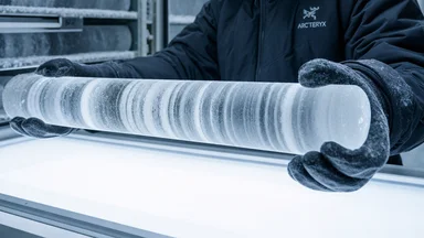
When you hold a slice of ice core up to the light, you see bands—some clear, some cloudy. These are annual layers, analogous to tree rings. In a perfect world, counting them gives you the age of each depth. But the world is not perfect. The assumption that each visible band represents exactly one year of accumulation is the first and most fragile link in the chain.

In Greenland, snow falls seasonally. Winter snow is typically finer and contains more dust, while summer snow is coarser and may show evidence of melting. But a single warm summer can melt the surface, erasing the seasonal signal. A wind event can deposit a crust that looks like a new layer but represents only hours. As depth increases, the weight of overlying ice compresses the layers, making them thinner and harder to distinguish. By 3,000 meters depth, annual layers may be only a few millimeters thick—beyond the resolution of the human eye.

For the GISP2 core, drilled in the 1990s, the original age model relied heavily on visual layer counting. The team counted roughly 110,000 layers to reach the bottom of the ice sheet, which they estimated to be about 110,000 years old. But later work using chemical markers and volcanic tie points suggested that some sections had been overcounted or undercounted by as much as 10–20%. A consistent 1% overcount would make a 10,000-year-old layer appear to be 10,100 years old—a shift that, when compared to other records, can change the inferred lag between CO2 and temperature by centuries.

The choice of age model thus becomes a critical decision. The GISP2 layer-counted chronology places the onset of the last deglaciation at roughly 14,700 years before present. A different model, tuned to the oxygen-isotope record from Antarctic ice, might place the same event 200 years earlier or later. Each choice carries implications for the timing of CO2 rise relative to temperature rise—a central question in understanding the carbon cycle's role in climate change.

How Two Age Models Tell Different Climate Stories

The most prominent alternative to layer counting is the use of oxygen-isotope tuning. Oxygen isotopes (δ¹⁸O) in ice reflect local temperature at the time of deposition. Because the δ¹⁸O signal is continuous and can be measured at high resolution, it provides a template that can be aligned with other records—for example, the δ¹⁸O from a different ice core or from marine sediments. This process, called tuning, assumes that the major climate events are synchronous across the region, an assumption that may or may not hold.

For the North Greenland Ice Core Project (NorthGRIP), two age models exist side by side. The first, known as the Meese–Dansgaard model, is based on layer counting and a few volcanic tie points. The second, called GICC05 (Greenland Ice Core Chronology 2005), combines layer counting with a more systematic use of volcanic markers and a Bayesian statistical framework to account for counting errors. The two models agree reasonably well for the past 10,000 years, but they diverge noticeably for older sections. For the Younger Dryas—a cold period that began roughly 12,900 years ago—the GICC05 model places the onset about 200 years earlier than the Meese–Dansgaard model.

That 200-year difference has consequences. The Younger Dryas is thought to have been triggered by a freshwater pulse from the melting Laurentide Ice Sheet, which disrupted ocean circulation. If the onset is earlier, the timing of that freshwater pulse relative to other records changes. It also affects the calculated rate of temperature change: a 200-year shift in a 1,000-year event changes the apparent steepness of the warming curve. A faster rate might imply a more sensitive climate system, while a slower rate suggests a more gradual response.

The paleoclimate community remains divided over which model is correct. Some argue that GICC05's use of multiple volcanic horizons—each tied to a known eruption date—makes it more reliable. Others point out that the volcanic markers themselves are not always precisely dated, and that the Bayesian adjustments can introduce artifacts. The debate is not academic: the IPCC's assessment of past climate sensitivity draws on these records, and a difference of 200 years in the timing of CO2 rise relative to temperature can change the inferred feedback strength by a factor of two.

The Physics That Makes Layer Counting Frail

To understand why layer counting is so challenging, it helps to consider what happens to a snowflake after it lands. Fresh snow is light and fluffy, with a density around 0.1 g/cm³. Over months, it compacts into firn, then into solid ice, reaching a density near 0.9 g/cm³ at about 100 meters depth. During this compaction, the annual layers thin nonlinearly. The uppermost layers may be tens of centimeters thick, but at 2,000 meters depth, a century of accumulation may be compressed into just a few centimeters.

Summer melting is the most common source of error. When the surface melts, water percolates downward and refreezes, creating a horizontal ice lens that can be mistaken for an annual layer. In some Greenland cores, melt layers are rare before the Holocene, but during the last interglacial period, summer temperatures were higher and melt layers are common. Counting errors in those sections can be severe. A 2012 study of the NEEM core in northwest Greenland found that visual layer counting overestimated the number of years by roughly 10% in sections with frequent melt layers.

Wind crusts are another problem. After a storm, wind can pack the snow surface into a hard layer that looks like a summer surface. If another snowfall follows quickly, the crust may be preserved as a false layer. Without chemical analysis to distinguish wind crusts from true summer surfaces, the counter can easily add extra years. One study estimated that wind crusts introduced an average overcount of 2–3% in the GISP2 core for the Holocene section.

Volcanic spikes are the gold standard for absolute dating. When a large eruption occurs—like the 1815 eruption of Mount Tambora in Indonesia—it leaves a layer of sulfate aerosols that can be detected in ice cores worldwide. By matching these layers to historically recorded eruptions, scientists can assign absolute dates. But only a handful of eruptions are large enough to leave a global signal, and for periods before written history, even those are uncertain. The 536 AD eruption, for example, is known from tree rings and historical accounts, but its exact source volcano is debated. For older sections, the only volcanic markers are those from large, well-dated eruptions like the 79 AD Vesuvius event, which provides a tie point but not enough to correct counting errors across the entire core.

Why Radiometric Dating Can’t Save Us Here

Given the problems with layer counting, one might ask: why not use radiometric dating? The answer lies in the material. Ice is mostly water, with trace amounts of dust, pollen, and dissolved gases. Radiocarbon (carbon-14) dating requires organic carbon—wood, charcoal, bone—that is virtually absent in ice cores. The tiny amounts of carbon in dust particles are often contaminated by modern carbon during drilling or handling, and the sample sizes needed are far larger than what a typical ice core section provides.

Uranium-series dating, which works well on speleothems (cave formations) and corals, is not applicable to ice because the uranium concentration is negligible. Argon-argon dating, used for volcanic rocks, requires minerals that crystallize at high temperatures—again, absent in ice. Even if we could date the ice itself, the decay of radioactive isotopes in water is too slow to be useful for the timescales of interest (tens of thousands of years).

The best cross-checks come from other archives. Marine sediment cores contain foraminifera that can be dated using oxygen-isotope stratigraphy and, in some cases, radiocarbon on shells. By matching the δ¹⁸O signal from ice cores to that from marine cores, researchers can transfer the marine chronology to the ice. This is the approach used by the INTIMATE (Integration of Ice Core, Marine, and Terrestrial Records) group, which aims to synchronize climate records across the North Atlantic region. The method works well for the last glacial period, where the δ¹⁸O signals are strongly correlated, but it introduces its own uncertainties. The marine chronology itself is not absolute; it relies on radiocarbon dating of foraminifera, which requires a calibration curve that extends only to about 50,000 years. Beyond that, the curve becomes less reliable, and the error bars widen.

In effect, paleoclimate dating is a chain of compromises. Each link—layer counting, volcanic markers, oxygen-isotope tuning, marine correlation—has its own systematic errors. The best age models combine multiple methods, but the choice of which method to prioritize can still shift the timeline by centuries.

A Case Study: The Abrupt Warming 14,700 Years Ago

One of the most studied climate events is the Bølling–Allerød transition, an abrupt warming that occurred roughly 14,700 years ago. In Greenland, temperatures rose by about 10°C within a few decades. The event is clearly visible in both the GISP2 and NorthGRIP cores as a sharp increase in δ¹⁸O. But the timing of this event relative to the rise in atmospheric CO2—which also occurred around that time—has been a subject of debate for over two decades.

Using the GISP2 layer-counted chronology, the CO2 rise appears to lag the temperature rise by about 800 years. This lag has been interpreted as evidence that CO2 was not the primary driver of the deglaciation; rather, changes in ocean circulation and albedo may have initiated the warming, with CO2 acting as a feedback. But when the same ice core data are placed on the GICC05 age model, the lag shrinks to roughly 200 years—within the uncertainty of the dating. A 200-year lag is consistent with CO2 playing a more active role, possibly amplifying the initial warming through the greenhouse effect.

Which is correct? It depends on which age model you trust. A 2014 study in Science used a new method—measuring the isotopic composition of argon in trapped air bubbles—to independently date the ice. The argon method suggested that the GICC05 model was closer to the truth, with a lag of roughly 200 years. But a 2018 paper in Nature argued that the argon method had its own biases, and that the layer-counted model could not be ruled out. The debate continues, with each camp publishing refinements to their methods.

The implications go beyond academic curiosity. The carbon cycle's sensitivity to warming is a key parameter in climate models. If CO2 rose 800 years after temperature, the feedback is weak; if it rose in 200 years, the feedback is strong. Models tuned to one scenario may overestimate or underestimate future carbon cycle responses. The uncertainty is not small: a factor of four in the lag translates to a factor of two in the implied carbon-cycle feedback strength, based on some estimates.

Additional Case Study: The 8.2 ka Event

Another example where dating choices matter is the 8.2 ka event, a cold period about 8,200 years ago caused by a freshwater outburst from glacial Lake Agassiz. In the GISP2 core, the event appears as a dip in δ¹⁸O, but its exact timing relative to the outburst varies by up to 150 years depending on the age model used. The GICC05 model aligns the event more closely with the outburst timing inferred from marine sediments, while the layer-counted model shows a delay. This discrepancy affects our understanding of how quickly the ocean circulation responds to freshwater forcing—a key parameter for predicting future changes in the Atlantic Meridional Overturning Circulation (AMOC).

Technical Details: Bayesian Age Modeling

To address these issues, modern age models like GICC05 and the upcoming ICC2026 use Bayesian statistics to combine multiple dating constraints. In a Bayesian framework, each observation (e.g., a counted layer, a volcanic marker, a δ¹⁸O tie point) is assigned a probability distribution. The model then finds the most likely chronology given all the data and prior assumptions about counting errors. For example, if layer counting suggests a certain depth is 10,000 years old, but a volcanic marker nearby gives an age of 10,200 years, the Bayesian model will adjust the chronology to a compromise, weighted by the reliability of each method.

One key advantage of Bayesian models is that they provide uncertainty estimates. Instead of a single age, each depth gets a range (e.g., 10,000 ± 50 years). This allows researchers to propagate uncertainty into their climate reconstructions. However, the Bayesian approach is sensitive to the choice of prior distributions. If the prior assumes that counting errors are small, the model will favor the layer-counted chronology; if the prior assumes larger errors, it will favor the volcanic markers. The community is still debating which priors are most appropriate, and different research groups use different assumptions, leading to slightly different chronologies.

What This Means for Future Paleoclimate Syntheses

Recognizing the problem, the paleoclimate community has launched several initiatives to harmonize ice core chronologies. The most ambitious is the Ice Core Chronology 2026 (ICC2026) project, which aims to produce a unified age model for Greenland and Antarctic cores covering the last 50,000 years. The project combines layer counting, volcanic markers, oxygen-isotope tuning, and Bayesian statistics to produce a single, best-estimate chronology with quantified uncertainties.

The goal is to achieve a ±50-year accuracy target for the entire 50,000-year span. That is a tall order: it requires reducing uncertainties by roughly a factor of two compared to current models. To reach it, the ICC2026 team is using a Bayesian framework that allows each dating method to contribute according to its reliability. For example, in sections with clear annual layers and no melt, layer counting is weighted heavily. In sections with melt or wind crusts, the Bayesian model downweights those counts and relies more on volcanic markers or oxygen-isotope tuning. The result is a chronology that is more robust than any single method alone.

But even the Bayesian approach cannot solve all problems. The model requires prior assumptions about the probability of counting errors, which are themselves uncertain. Different choices of priors can shift the final chronology by 50–100 years in some sections. The community is still debating which priors are most defensible. As of late 2024, a draft of the ICC2026 model has been circulated, but it has not yet been adopted as a standard.

The IPCC's Sixth Assessment Report (AR6) already acknowledges age-model uncertainty as a source of spread in paleoclimate reconstructions. Future reports will likely need to incorporate multiple age models in their assessments, rather than relying on a single best estimate. This is a shift from previous practice, where a single chronology was often used without explicit discussion of alternatives. For a non-specialist, the takeaway is that every number in a paleoclimate study carries a procedural choice. The same core can tell different stories depending on how we count its layers.

The Takeaway for Non-Specialists

If you read a news article claiming that CO2 lagged temperature by 800 years during the last deglaciation, ask: which age model was used? If the article does not mention the dating method, it is likely relying on a single, perhaps outdated, chronology. The same data, processed with a different model, might show a 200-year lag. The uncertainty is not a flaw; it is a honest reflection of the difficulty of the task.

Paleoclimate science is not unique in this regard. Similar debates arise in other fields that rely on dating—tree-ring chronologies, radiocarbon calibration, and sediment core analysis. A recent replication study in another context showed how procedural choices can alter results. The key is transparency. When researchers explicitly state their dating assumptions and discuss the alternatives, the science becomes stronger. When they do not, the results can appear more certain than they are.

The next time you see a graph of past temperature and CO2, remember that the x-axis is not a given. It is a constructed timeline, built from fragile layers and human judgment. The story it tells depends on the choices made in the lab, and those choices are still being debated. That uncertainty is not a weakness—it is a sign that the science is alive and questioning itself.

For those interested in a deeper dive, a related piece on drill core sampling rates explores how even the way we extract ice from the ground can affect the data we get. And a multi-laboratory replication test in a different field shows that the problem of procedural sensitivity is widespread across science.

Looking ahead, the paleoclimate community faces a crucial challenge: can we reduce age-model uncertainty enough to answer the big questions about carbon cycle feedbacks? The ICC2026 project is a step in that direction, but it will require continued collaboration and methodological innovation. Perhaps the most important lesson is that uncertainty is not a barrier to understanding—it is a guide to where more work is needed. The next decade will determine whether we can tighten the timeline enough to resolve the CO2-temperature lag debate once and for all.